NVIDIA leverages data science and machine learning to optimize chip manufacturing and operations workflows—from wafer fabrication and circuit probing to packaged chip testing. These stages generate terabytes of data, and turning that data into actionable insights at speed and scale is critical to ensuring quality, throughput, and cost efficiency. Over the years, we’ve developed robust ML pipelines that tackle problems like defect detection and test optimization.
This is the first in a series of blogs that will share our key learnings from deploying such pipelines using CUDA-X libraries like NVIDIA cuDF and NVIDIA cuML. While these lessons come from semiconductor manufacturing, the challenges and solutions are widely applicable across logistics, quality engineering, and supply chain optimization.
Let’s start with a real-world classification task: predicting whether a chip will pass or fail a specific test. In more advanced scenarios, the objective extends to predicting a chip’s performance bin—from L1 to L5—and formulating the problem as a multi-class classification problem.
In both cases, the model consumes rich measurement signals from multiple sources:
- Sparse features: wafer-level metrology
- Dense signals: die-level data from circuit probe (CP) tests, and high-fidelity functional test (FT) results from packaged units
These datasets often span hundreds of thousands of rows and several hundred features, quickly overwhelming traditional CPU-bound data processing workflows.
Tackling imbalanced datasets
A key challenge in operations-focused ML (Ops ML) is extreme class imbalance. In some chip families, more than 99% of units pass a test, leaving only a fraction that fail. This skew makes training robust models difficult, as standard learners tend to bias toward the majority class.
To address this, we leverage CUDA-X data science libraries, including cuDF and cuML, for rapid data transformations and scalable model experimentation. When dealing with such highly imbalanced datasets, we apply targeted sampling methods—including Synthetic Minority Over-Sampling Technique (SMOTE) and undersampling—to balance the classes, thus enabling more stable and effective model training. Leveraging CUDA-X libraries, these strategies can be done directly in GPU memory, drastically reducing iteration times and scale experiments seamlessly.
Synthetic minority oversampling technique (SMOTE)
# Minority Oversampling (SMOTE) using cuML
from imblearn.over_sampling import SMOTE
from cuml.neighbors import NearestNeighbors

# X,y are dataframes with features and target resp.
nn = NearestNeighbors(n_neighbors=6)
X_resampled, y_resampled = SMOTE(n_neighbors=nn).fit_resample(X, y)
In our experiments, cuML’s NearestNeighbors when compared to native scikit-learn, in conjunction with SMOTE, shows speedup of 2x to 8x demonstrating the value of CUDA-X libraries.
Stratified undersampling
# Quick example of stratified sampling using cuDF
df['label'] = df['label'].astype('category')
sampled_df = df.groupby('label').sample(n=10000, replace=True)
X_resampled, y_resampled = sampled_df[x_features], sampled_df[target]
In practice, rapid iteration is critical. We’ve often gone from raw CP and FT data to model-ready features in hours instead of days—thanks to cuDF’s GPU-accelerated joins, filters, and groupbys. And when training models like random forests or XGBoost, cuML consistently offers 5x to 30x speedups over CPU-based versions, allowing us to test more hypotheses and tune models faster. This agility has made it feasible to prototype solutions with engineers on the fab floor in near real time.
Metrics that matter for evaluation
Highly imbalanced datasets not only complicate training—they also distort standard metrics for evaluation. For example, accuracy becomes a meaningless metric when a model can predict “pass” for every chip and still be 99% correct.
To better reflect true performance, we rely on metrics like weighted accuracy and area under the precision-recall curve.
Weighted accuracy
We evaluate accuracy for each category separately and take a weighted average to give each category equal importance and remove the imbalance.
Pass accuracy: p_ac = Predicted Pass/(Predicted Pass + True Pass)
Fail accuracy: f_ac = Predicted Fail/(Predicted Fail + True Fail)
The weighted form is:
acc = w_f * f_acc + (1 – w_f) * p_acc
A default and convenient choice for most settings is w_f = 0.5, giving
acc = ( f_acc + p_acc ) / 2
Precision-recall curve
In severely imbalanced datasets, the traditional relative-operating-characteristics (ROC) curve and area under ROC curve metrics can be misleading. For example, consider a heavily imbalanced dataset with 98% yield throughput, i.e., 2% of parts “fail.”
Let us compare the ROC and precision-recall curves. The marker on the ROC curve highlights a point with a true positive rate of 0.61 and a false positive rate of 0.13. At first glance, this might seem like a reasonable operating point. However, for imbalanced datasets (like the one shown below, where most outcomes are “pass”), ROC curves can be misleading because they don’t emphasize the cost of false positives.
Look at the same point on the precision-recall (PR) curve. Here, the precision is just 0.09, and the recall is 0.61. This tells us that for every 100 units the model predicts as “fail,” only 9 are truly failing—which isn’t acceptable for most real-world manufacturing scenarios where the cost of acting on a false alarm is high.
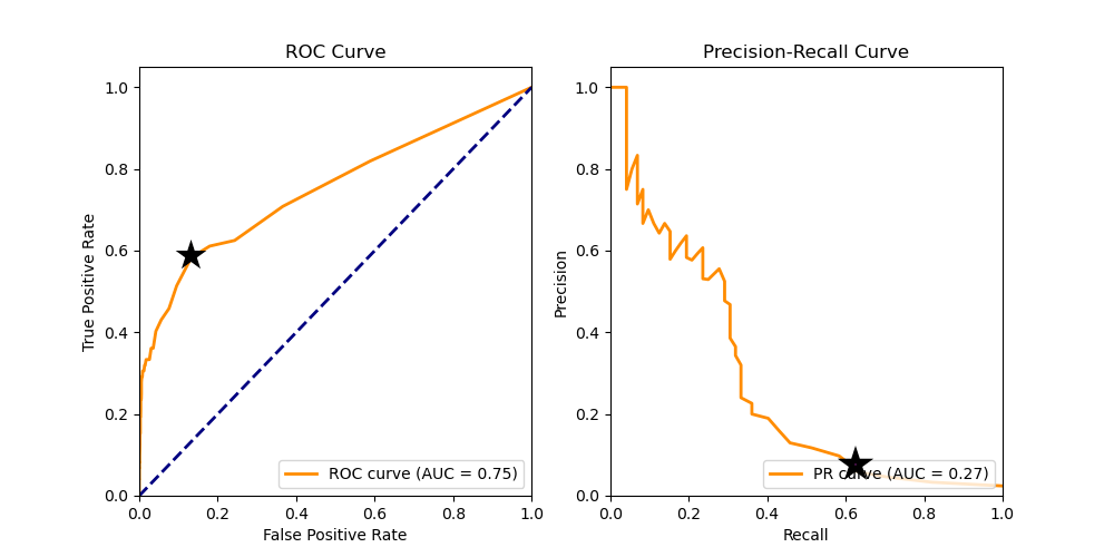
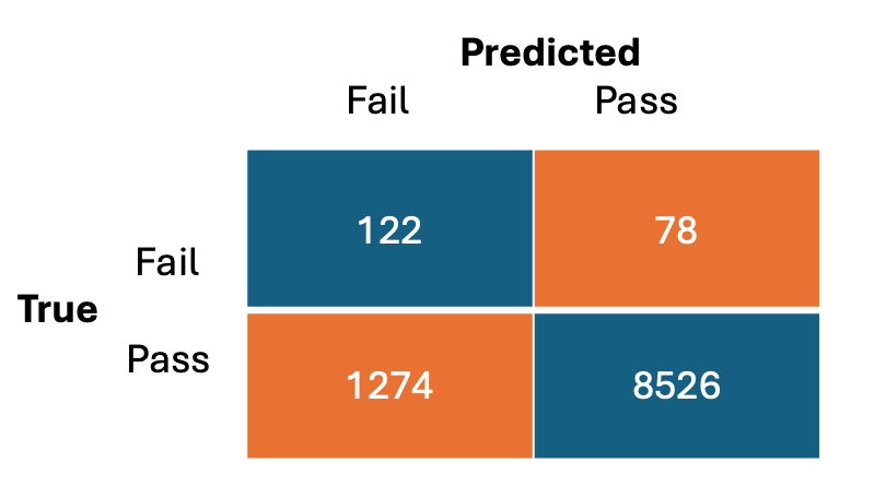
The confusion matrix below—which corresponds to the marker on the plots above— reinforces this. At the selected operating point, 1,274 units were incorrectly flagged as “fail,” compared to just 122 correctly flagged ones. That’s a false-alarm rate of over 90%. The precision-recall curve makes this poor performance much more visible.
Here is the code for the discussed scenario.
import cuml
from sklearn.datasets import make_classification
from cuml.model_selection import train_test_split
from cuml.ensemble import RandomForestClassifier as cuRF
from cuml.metrics import roc_auc_score, precision_recall_curve
import cupy as cp
from sklearn.metrics import roc_curve, auc
import matplotlib.pyplot as plt

# synthetic dataset dimensions
n_samples = 10000
n_features = 20
n_classes = 2

# random forest depth and size
n_estimators = 25
max_depth = 10

# generate synthetic data [ binary classification task ]
X, y = make_classification (n_classes = n_classes,
                        n_features = n_features,
                        n_samples = n_samples,
random_state=13,
                       weights =[0.98, 0.02]))
X_train, X_test, y_train, y_test = train_test_split(
X, y, random_state = 0, test_size=0.3)
# Train the RandomForest Classifier
model = cuRF( max_depth = max_depth,
          n_estimators = n_estimators,
          random_state  = 0)

trained_RF = model.fit ( X_train, y_train)
ypred = model.predict_proba ( X_test) [:, 1]

# Calculate the ROC curve
fpr, tpr, _ = roc_curve(y_test, ypred)
roc_auc = roc_auc_score(y_test, ypred)
plt.plot(fpr, tpr, color='darkorange', label='ROC Curve')

# Calculate the Precision-Recall curve
precision, recall, _ = precision_recall_curve(y_test, ypred)
pr_auc = auc(cp.asnumpy(recall), cp.asnumpy(precision))
plt.plot(recall, precision, color='darkorange', label='Precision-Recall Curve')
Interpretability
Model performance is only part of the story. In operational settings, interpretability and actionability are equally important. Predicting test outcomes has real value only when domain experts can understand and trust the model’s reasoning.
That’s why we rely on cuML’s native support for feature importance in ensemble models. This capability helps us surface high-impact features for engineering review. In some cases, these insights have led to the identification—and elimination—of redundant or low-value test steps, directly translating into cost savings and streamlined processes.
Another way domain experts can reason through model outputs is with cuML’s GPU-accelerated SHAP (SHapley Additive exPlanations) implementations, such as the Kernel SHAP and Permutation SHAP explainers. These tools enable us to understand the contribution of each feature to the model’s predictions, providing both global and local interpretability. In practice, these SHAP-based insights have helped us identify test steps that were redundant or less predictive, leading to cost savings through test elimination.
Conclusion
For those interested in exploring further, the cuDF documentation provides comprehensive guides on GPU-accelerated data manipulation, while the cuML documentation details the suite of machine-learning algorithms optimized for GPUs. These resources are invaluable for practitioners aiming to harness the full potential of CUDA-X Data Science libraries in their workflows.
If you already have workflows built out using libraries like pandas, Polars, or scikit-learn, CUDA-X also offers drop-in, zero-code-change acceleration through cuDF’s pandas accelerator and cuML’s estimators for scikit-learn. This makes it easier than ever to scale up your existing Python pipelines without rewriting them from scratch. To dive deeper into accelerated data science, you can enroll in hands-on courses from our DLI Learning Path.
In our upcoming blogs, we’ll explore feature engineering techniques like coalescing test signals and calculating spatial Z-yield, model evaluation with business-aware metrics like the Cost of Quality (CoQ) curve, and best practices for using ML to augment and empower operations engineering. These lessons are grounded in CUDA-X-based pipelines and NVIDIA’s manufacturing domain, but the patterns are repeatable in any data-rich, decision-driven operations environment.
Stay tuned as we walk through the next stages of building and deploying ML for Ops—accelerating data processing workflows is only the beginning. Making it actionable is where the real value lies.